Module Projects

Year 1: RoboDK Offline Programming

RoboDK is a powerful offline programming software that supports many robot brands, with a library of over 500 robots from more than 50 manufacturers including ABB, KUKA, Fanuc, Motoman, and Universal Robots. It can generate real robot programs in the syntax required by each brand. This project focused on simulating three common robotic tasks: milling (Figure 1), welding (Figure 2), and deburring (Figure 3). For the simulation, I selected the ABB IRB 120-3/0.6, a 6‑DOF robot well suited to precise operations in limited spaces. The tasks were carried out by manually teaching the arm using RoboDK’s jogging tools.

Each task began with setting up the station, including the robot, frames, target points, and tools imported from RoboDK’s library. Frames define the orientation and position of targets. I chose to assign the reference frame to the work table so that, if the table is moved, only recalibration of the frame is required. Using the robot as the frame would mean re‑teaching all points, while assigning it to the object works best for single‑part setups but is inefficient in batch production. Since my aim was to simulate a multi‑part process, the table frame was the most practical choice.

The TCP (tool centre point) was also given a frame; this refers to the operating position and orientation of the tool with respect to the robot flange (the tip of the robot). Examples include the tip of a welding gun or the midpoint between gripper fingers. The TCP should match the target positions when the robot is in operation. Once this stage was complete, the robot was then given the target points by moving it to each desired position and declaring it a target. Approach and retract positions were also included to ensure collision‑free motion. I did encounter difficulties with singularities, as seen in the deburring video at 0:15, which led to some inefficient movements.

Year 1: Pick and Place Robot Arm

This project focused on building and controlling a 4‑DOF robot arm. An Arduino Duemilanove‑inspired “BotBoarduino” was used as the microcontroller, and HiTec servo motors were used to drive each joint. There were three main tasks, including an inverse kinematics task in which the arm’s end effector had to follow a horizontal linear motion of 5 cm in both the positive and negative x‑directions. The project concluded with a pick‑and‑place task, demonstrated by our team’s robot in the video above. We used a geometric approach to inverse kinematics to obtain the required joint angles for the pick‑and‑place motion. The cubic polynomial and function definitions used were as follows:

A for loop was used to compute 50 trajectory points for x, y, and z between the initial and final positions, with the loop iterating from t = 0 to t ≤ t_f in steps of 0.1 seconds. The cubic polynomial function above was used to calculate the coordinates at each time step along the trajectory. The Set_Position member contains the inverse kinematics routine, which calculates the joint angles required to actuate the motors. Within the loop, a 100 ms delay was added so that the total motion time was 5 seconds. Target points were defined as home, pick, and place positions, and the robot was programmed to move in the sequence home → pick → home → place → home. The header, source, and sketch files for the project are attached below.

Year 2: Image Processing and Object Detection Project

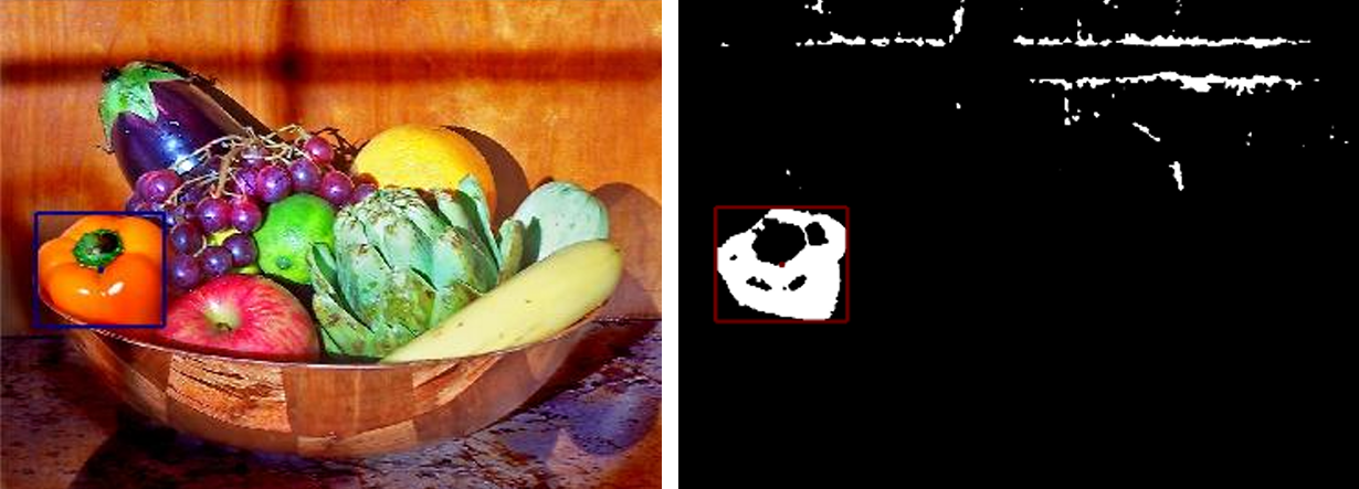
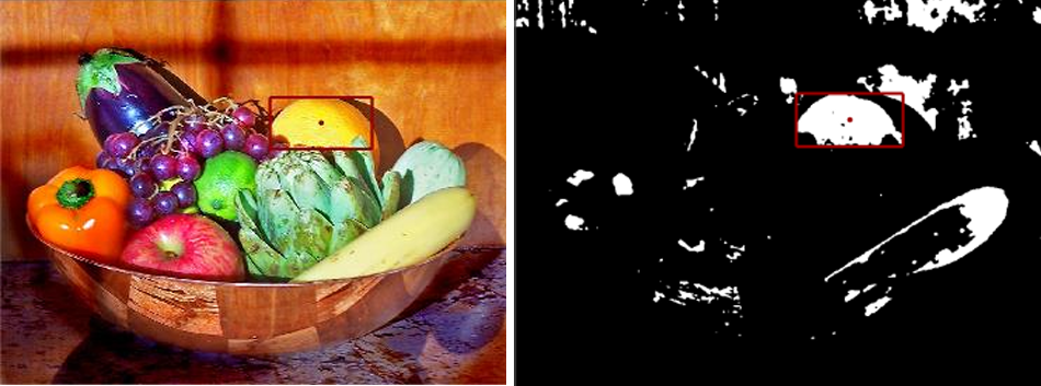
This was the first project of my second year on this elective module. It built on image‑processing fundamentals such as thresholding, Gaussian filters, median filters, and Sobel filters, as well as methods for finding an object’s centroid and orientation in an image. The project consisted of two tasks: the first required identifying the centroids and drawing bounding boxes around different fruits in a given image, and the second involved determining the centroid, orientation, and perimeter of an object in another image.

Once the image was pre‑processed, I applied a connected‑components algorithm based on a breadth‑first search. This method starts from a given pixel and checks its eight neighbours; any neighbour that is part of the same object is assigned the same label as the original pixel. This efficiently groups connected pixels into distinct regions, which in this case corresponded to different fruits in the image. The largest connected regions in each area matched the capsicum, apple, and lemon specified in the task, and the algorithm successfully identified all three fruits.

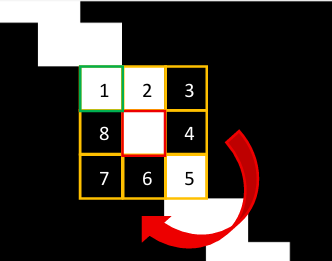
The next part of the task focused on identifying the orientation and centroid of an object within an image. Since the image had a clear intensity difference between foreground and background, only thresholding was required for preprocessing. To determine the centroid, image moments were used to calculate the weighted average of pixel intensities. The orientation was computed using second‑order image moments. Additionally, the eigenvalues and eigenvectors were used to construct the inertia matrix, which defines the major and minor axes of the object. To calculate the perimeter, a Sobel filter was first applied to extract edges. Once the edges were detected, the Moore–Neighbour tracing algorithm was used, which follows the 8‑connected neighbours around the boundary pixels. Previously, I used a simpler method that always chose the top‑left high‑intensity neighbour in a 3×3 grid, which sometimes caused the algorithm to loop incorrectly and miscalculate the perimeter. The Moore–Neighbour method avoids this by considering the previous neighbour’s position and starting two positions before it, effectively “hugging” the object boundary and producing the correct perimeter. The images below show the analysed object, including the region that previously caused issues with perimeter calculation. The code for both tasks is provided below and can be downloaded to see the implementation in action.